Insights from the RAPID–MOCHA observation network in the North Atlantic have motivated a recent focus on the South Atlantic, where water masses are exchanged with the neighboring Indian and Pacific ocean basins. Moreover, the South Atlantic meridional overturning circulation basin-wide array (SAMBA) was recently launched to monitor variability in the South Atlantic MOC (SAMOC) at 34.5\(^\circ\)S. In this work, we were interested in understanding the processes which generate volume transport variability that would be observed at this latitude band.
The ECCO State Estimate
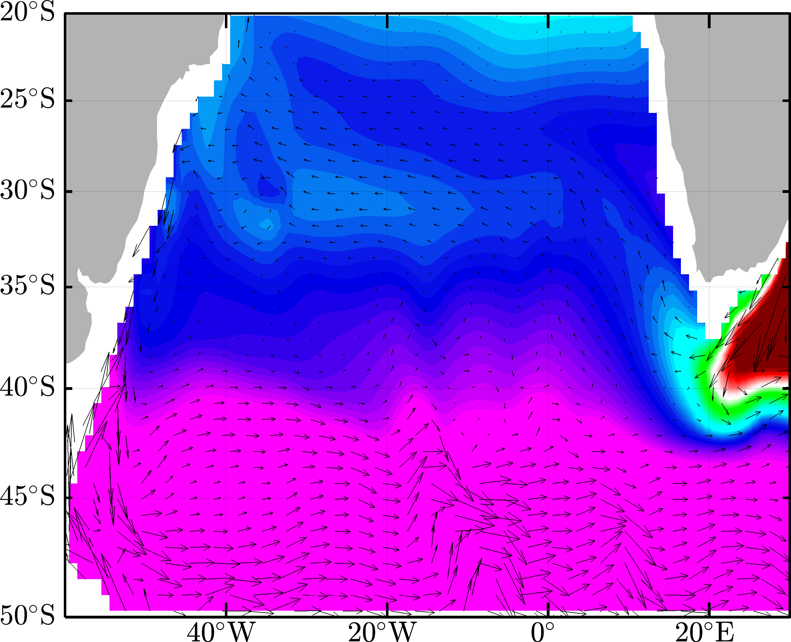
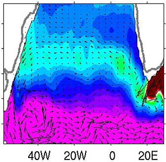
We made use of ECCOv4r2: a state estimate generated by the consortium for Estimating the Climate and Climate and Circulation of the Ocean (ECCO). Importantly, this model is constrained to a vast array of ocean observations over the past two decades (Forget et al. 2015) and provides a relatively realistic view of the South Atlantic, a region which hosts complex water mass exchanges (e.g. Garzoli & Matano 2011). See, for example, a comparison of temperature from ECCOv4r2 and a gridded Argo product in the region.
| ECCOv4r2 | Argo | |
|---|---|---|
 |
 |
 |
| from Dong et al. (2014) used with permission from John Wiley and Sons. |
This shows time mean temperature at 1000m depth, where the Argo figure is taken from Dong et al. (2014). The match is not perfect, but it is quite close and gives us confidence that the model has water masses more or less in the right place. Check out the paper, Smith and Heimbach (2019) for a more detailed comparison to Argo estimates. See Dong et al. (2014) for an in depth comparison of Argo to commonly used climate models and a great discussion, for instance, on the importance of having the Brazil-Malvinas Confluence at around 38\(^\circ\)S.
Sensitivity analysis to uncover ocean dynamics
Another key advantage of using the ECCO state estimate (and the MITgcm in general) is for access to an adjoint model, which provides a computationally tractable means to perform a comprehensive sensitivity analysis. Here we compute sensitivities of the SAMOC at 34\(^\circ\) S to atmospheric state variables (e.g. wind stress, precipitation).
 Here we see the sensitivity of the SAMOC to zonal wind stress at one month lead time,
where
increasing westerlies over red regions would increase the monthly mean SAMOC
one month later, and vice versa for blue.
This figure shows some interesting features worth noting.
Here we see the sensitivity of the SAMOC to zonal wind stress at one month lead time,
where
increasing westerlies over red regions would increase the monthly mean SAMOC
one month later, and vice versa for blue.
This figure shows some interesting features worth noting.
- The thick band of positive sensitivity around 30-40\(^\circ\)S mostly corresponds to Ekman dynamics, where an increase in the westerlies would generate net mass transport to the left in the Southern Hemisphere, and hence an increase in Northward surface transport and the SAMOC.
- The negative sensitivity near the equator corresponds to Kelvin wave propgation, where a westerly perturbation would generate a pressure anomaly which travels cyclonically along the Eastern boundary to 34\(^\circ\)S in approximately one month. The resulting horizontal pressure gradient causes a decrease in northward geostrophic transport.
- The patterns largely correspond to topographic features which act as wave guides, steering pressure anomalies generated by wind stress perturbations to 34\(^\circ\)S.
- The sensitivity shows that the domain of influence for the SAMOC is quite broad, covering neighboring ocean basins on short timescales. This result differs from what has been shown in the North Atlantic, where AMOC variability on interannual timescales is shown to largely be governed by dynamics confined to that basin (Pillar et al. 2016).
Reconstruction of SAMOC variability and attribution
Finally, we convolved the sensitivities with historical forcing variability from ERA-Interim in order to reconstruct the monthly SAMOC variability. This operation can be conceptualized as a high dimensional taylor expansion:
\[\delta MOC \simeq \frac{\partial MOC}{\partial F} \, \delta F\]where \(\delta F\) is the atmospheric forcing variability. The reconstruction is shown below, providing some verification that the linearized sensitivities capture most of the variability in ECCO’s representation of the SAMOC.
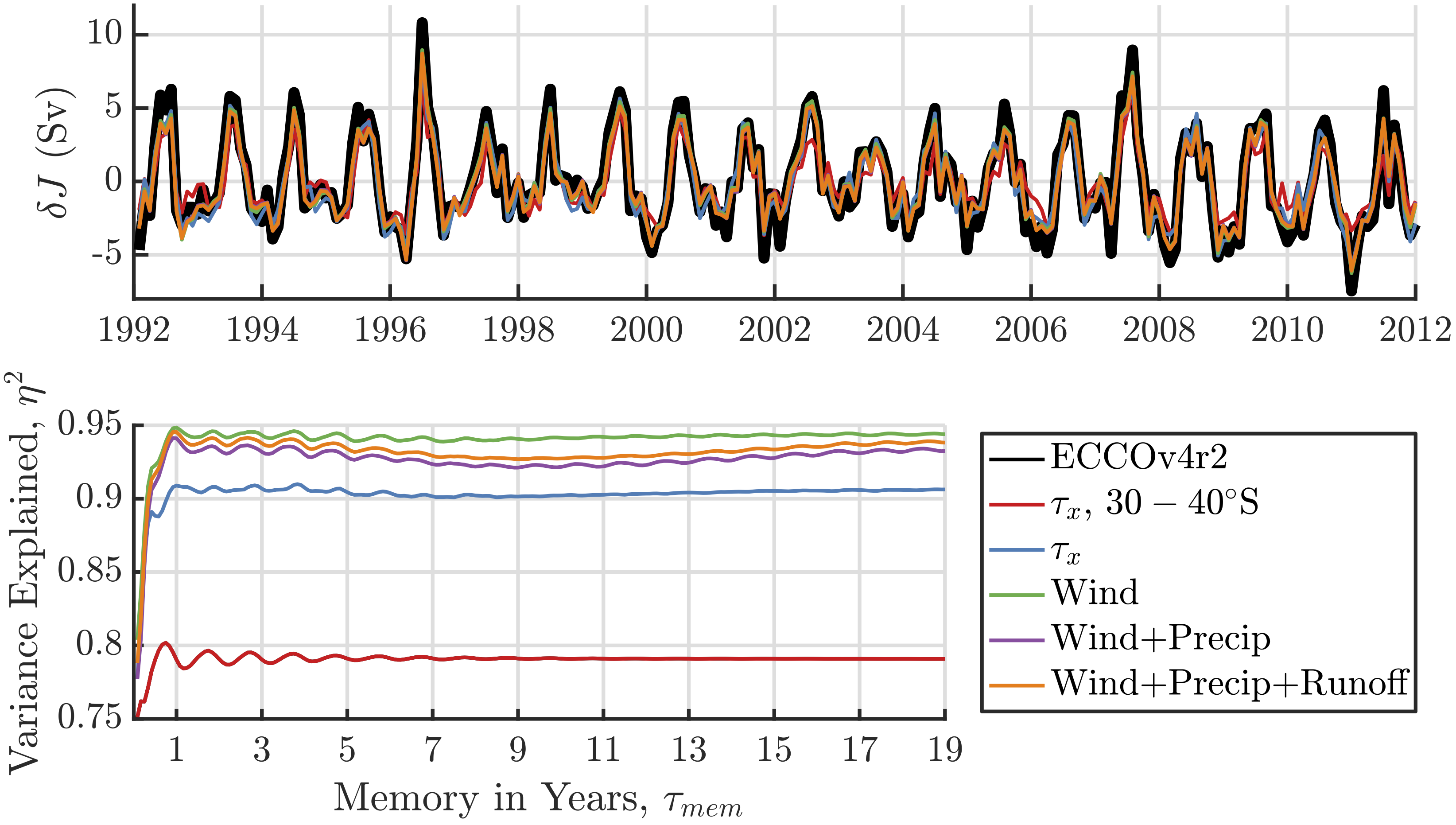
The black line shows the SAMOC computed by the nonlinear forward model (i.e. the full GCM), and each of the colored curves show various reconstructions using adjoint-derived sensitivities. For instance, the red curve shows a reconstruction where only the sensitivity to zonal wind stress between 30-40\(^\circ\)S is used, while the blue curve contains global zonal wind variability. The “memory” axis for the variance explained curve shows how many months of lead time in the sensitivities are included in the convolution. For example, a time series reconstructed from global zonal wind variability with only one month of lead time is computed by “pointwise-multiplying” the sensitivity map shown earlier with ERA-Interim wind variability at one month prior to the given month being reconstructed.
This figure provides verification and hints at some interesting results we obtained by restricting the convolution to various forcing variables and regions of the world (as is shown for e.g. the red vs blue curves above). Some highlights of the results are:
- The seasonal cycle of the SAMOC is largely driven by local zonal wind forcing. Because the seasonal cycle in the 20 year signal is quite large compared to any interannual variability, zonal winds do a good job of capturing variability in the 20 year record as well (see red curve above).
- Wind stress acts on relatively short timescales and the majority SAMOC variability can be attributed to forcing over one year of lead time. This is shown in the figure above as the explained variance is quite high even when the reconstruction only considers atmospheric variability a few months to one year in advance.
- Interannual variability is the result of a much more complex balance of forcing from various components (buoyancy forcing plays a bigger role), and from remote regions of the world (including a nontrivial component originating from the tropical Pacific).
For more details, please see:
Smith, T., & Heimbach, P. (2019). Atmospheric Origins of Variability in the South Atlantic Meridional Overturning Circulation. Journal of Climate, 32(5), 1483–1500. https://doi.org/10.1175/JCLI-D-18-0311.1
References
Dong, S., Baringer, M. O., Goni, G. J., Meinen, C. S., & Garzoli, S. L. (2014). Seasonal variations in the South Atlantic Meridional Overturning Circulation from observations and numerical models. Geophysical Research Letters, 41(13), 4611–4618. https://doi.org/10.1002/2014GL060428
Forget, G., Campin, J.-M., Heimbach, P., Hill, C. N., Ponte, R. M., & Wunsch, C. (2015). ECCO version 4: An integrated framework for non-linear inverse modeling and global ocean state estimation. Geoscientific Model Development, 8(10), 3071–3104. https://doi.org/10.5194/gmd-8-3071-2015
Garzoli, S. L., & Matano, R. (2011). The South Atlantic and the Atlantic Meridional Overturning Circulation. Deep Sea Research Part II: Topical Studies in Oceanography, 58(17), 1837–1847. https://doi.org/10.1016/j.dsr2.2010.10.063
Pillar, H. R., Heimbach, P., Johnson, H. L., & Marshall, D. P. (2016). Dynamical Attribution of Recent Variability in Atlantic Overturning. Journal of Climate, 29(9), 3339–3352. https://doi.org/10.1175/JCLI-D-15-0727.1